Forecasting for Sugar Bon‐Bon Cereals

Objective

Formulation & testing of different exponential models on the product data.

Introduction

You are working for a retailer that sells a lot of breakfast cereals. One of the cereals that you sell is the popular Sugar Bon‐Bon brand that features twice the sugar and even more caffeine.

Visualization of raw data

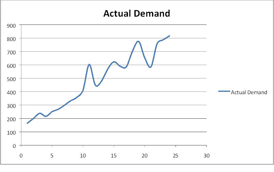
Simple Exponential Smoothing (SES)

We know that SES assumes stationary demand. i.e. it forecasts does not take into account trends or seasonalities. Even so, we would still like to know the effect of using SES on the forecasts.

Underlying model: \(x_{t} = a + e_{t}\)

Forecasting model: \(\hat{x}_{t,t+1} = \alpha x_{t} + (1 – \alpha) \hat{x}_{t-1,t}\)

Where \(\hat{x}_{t,t+1}\) is forecast for the next period, \(x_{t}\) is the present actual demand and \(\hat{x}_{t-1,t}\) is forecast for the previous period.

Initialization of the parameters

There are many ways of doing this. We can take the centered average for the first 4 or 5 periods. We can also take the average of the first 3, 4 or 5 periods depending on the data.

We take \(\hat{a}_{4,5}\)=205.25

We take α=0.15

Using the above model, the forecast for period 25 is around 654 bars. Also the forecast for period

30 will also be the same i.e. 654 since the model assumes stationary demand.

MAPE for SES is 0.279329

Holt’s Model (HM)

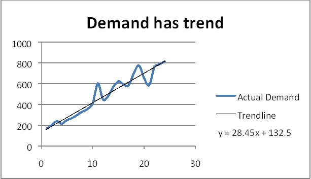
Since the data shows a positive trend, we use HM which assumes level & trend.

Underlying model: \(x_{t} = a + bt + e_{t}\)

Forecasting model: \(\hat{x}_{t,t+\tau} = \hat{a}_{t}+\tau \hat{b}_{t}\)

Updating Component:

\(\hat{a}_{t}=\alpha \hat{x}_{t}+ (1-\alpha)\hat{x}_{t-1,t}\)

a^t = α xt + (1 – α) x^t‐1,t

\(\hat{b}_{t}=\beta (\hat{a}_{t}-\hat{a}_{t-1})+(1-\beta) \hat{b}_{t-1}\)

b^t = β (a^t ‐ a^t‐1) + (1 – β) b^t‐1

Initialization of parameters

We take α = 0.2 and β = 0.05

We take \(\hat{a}_{t}\) = 157.5 & \(\hat{b}_{t}\) = 19.1

Comparison of models

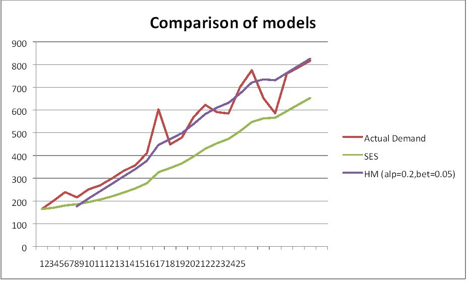
MAPE of the various models

	MAPE
SES	0.279329
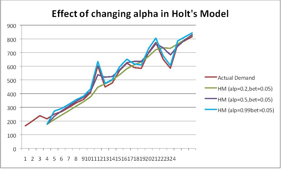
HM (alp=0.2bet=0.05)	0.128729
HM (alp=0.5bet=0.05)	0.120443
HM (alp=0.99bet=0.05)	0.112559

The MAPE and various other measures such as RMSE or MAD or most any other metric will improve as we increase the value of Alpha. This does not mean we are getting a better model. This means is that we are only fitting the model better to the historical data that we have. We are simple placing more weight to the most recent observations. Therefore, we should monitor effect of alpha & change as and when required.

Conclusion

Holt’s model with alpha=0.2 seems to be best way to forecast the demand of sugar cereals.